Panels User Guide

Many people have contributed to this document, including: Mark Frye, Michael Reiser, Michael Dickinson, Stephen Holtz, Chuntao Dan, Sung Soo Kim, John Tuthill.

This version of the document, compiled in June, 2022, leverages the Generation 2 User Guide to the Modular LED Display Generation 3. It was primarily written as a guide to students in the Neural System and Behavior Course.

The technical basis for Modular LED Displays Generation 4 is very different, there is an extensive documentation available as part of this website. If you don’t find what you are looking for, please get in contact.

Introduction

The flight arena is a powerful tool for addressing questions about sensory control of behavior, and when paired with genetic techniques, can be an equally powerful tool for probing neural circuits. This document offers an introduction to the flight arena and should serve as a reference when starting to run experiments. It contains a brief history, an overview of some of the physical components on the arena, and documentation on arena operation from a computer (see the outline below). Troubleshooting, assembly and required downloadable content are all available on the Modular LED Display Website:

Throughout the document we tend to refer to the tiled LED array as the arena, composed of individual panels, the image they display as patterns, and the black box that gives it all life as the controller.

Outline

The rest of the documentation will be divided into the following sections:

• History and Principles of Operation – Background and principles of arena operation.
• Fly Preparation – Fly housing and tethering with some helpful tips.
• Hardware Overview – The common physical components of an arena.
• Software Operation – Detailing the components of software for experiments.
• Example Experiments – Using a simple tutorial.
• __Technical Appendices – For more software specific commands and operation.

History and Principles of Operation

The devices and techniques described in this document owe much to approaches developed at the Max Planck Institute for Biological Cybernetics in Tübingen, Germany. This institute grew in the early 1960s around a group of four scientists: Werner Reichardt, Karl Götz, Valentino Braitenberg, and Kuno Kirschfeld, who adopted the visual system of flies as a general model system for neural processing. The term Biological Cybernetics was used to describe the use of information theory, computer science, control theory, etc. to characterize biological systems. The term reverse engineering is often used today to describe similar approaches. This enterprise generated a remarkable body of work, which ranged from detailed anatomical descriptions of visual system circuitry (e.g. discovery of ‘neural superposition’ in the fly) to sophisticated behavioral and physiological measurements (e.g. characterization of the lobula plate tangential cell system), to development of mathematical models of neural processing (e.g. refinement of the Hassenstein-Reichardt elementary movement detector model).

Perhaps less appreciated, was the work of Karl Götz, who developed an ingenious set of experimental methods for studying the optomotor control of flight in the fruit fly, Drosophila melanogaster. The work influenced not only the techniques described here, but also served as the direct foundation for many recent studies of visual spatial memory in Drosophila. The focus of his pioneering work was to produce visual stimuli with specific spatial and temporal properties, record the resultant behavioral responses, and then derive the intervening transfer functions. By formalizing the functional relationships between visual input and motor output, he was able to develop and test specific hypotheses about the underlying neural structures. The work was made enormously challenging because there was no off the shelf instrumentation for such experiments. Götz literally drew the plans for the devices he used throughout his career, often leaving them on the desk of the chief institute machinist before walking home in the early hours of the morning. Götz spent equal time developing ingenious ways of presenting visual stimuli to flies, and clever ways of recording, quantitatively, how the flies responded. One early device was a complex braid of fiber optic filaments that took the images displayed on an analog oscilloscope and wrapped them into a cylinder surrounding the fly. Another device employed active electromechanical feedback to record the yaw torque generated by a tethered fly. One of his more ingenious experimental techniques was a system that optically tracked the beating wings of a tethered fly, and electronically coupled these signals to rotation of a spinning glass disk, such that light projected through fish-eye optics created a pattern of stripes and spots on a circular cylinder surrounding the fly. As the fly (suspended in the middle of a rotating striped drum) tried to turn left, bilateral changes in wing stroke amplitude triggered servomotors to rotate the drum to the right. Under these conditions, the fly has closed-loop control over the visual panorama. Using such systems, Götz pioneered studies that linked the responses of the flies visual system to its motor responses in the form of muscle activity, wing motion, and aerodynamic forces.

Recent technical advances have made flight simulators easier to build and more sophisticated, but the basic architecture remains: present a visual stimulus to the fly, record what it does (in open loop), or provide it with the opportunity of controlling what it sees (in closed loop). The new systems are modular and fully programmable for visual images of varying brightness, contrast, and spatial layout.

Fly Preparation

Housing Flies

For normal, wild-type experiments, flies are generally stored in incubators at fixed temperatures on a regular light cycle. For example flies may be stored at 25° C with lights on from midnight to 4 pm. The following are some guidelines and tips on storing flies.

• Flies are crepuscular animals with activity peaks in the early morning and late afternoon – when it is cool enough to fly and light enough to see. One popular approach is to time experiments when flies are most active. Flies should be kept on a regular light:dark cycle and perform experiments during their crepuscular peaks. The afternoon peak is typically the most convenient. This requirement is relaxed at MBL. Our flies will still entrain to the daily rhythms of the lab, albeit with a peculiar light:dark cycle.
• It is quite helpful to use flies reared at low density. Presorting flies a day or two before running the experiment seems to improve flight time in some stocks.
• Laboratory stocks which have reproduced for some time in vials can, over time, begin to fly less reliably than freshly caught and established lines. If possible, crossing two lab stocks can result in very high-performance flies.

Tethering Flies

The most critical step in collecting high quality data in a flight simulator is tethering the animals. Well-chosen, healthy, properly-tethered (i.e. happy) flies will generate hours of data each day. Crappy flies (sensu Reiser), poorly tethered are not worth putting in the arena.

Once you have chosen a healthy batch of flies (see Housing Flies and Effectively Using Flies), the next step is to tether them. In brief, a batch of flies is transferred from a bottle to a small vial that is inserted in a brass block on a cooling stage set at about 4°C. The low temperature anesthetizes the flies within 30 seconds or so. The flies may then be sprinkled on the surface of the cooling stage. Choose a large, healthy-looking fly (usually a female) with wings nicely folded back over its abdomen for transfer to the socket of the sarcophagus using a suction wand. The trickiest part of the process is coaxing a fly into proper position within the sarcophagus using a fine brush. Ideally the fly will remain in place in the bottom of the sarcophagus, but gentle suction can also be used. The fly is then tethered to a fine tungsten pin using UV-activated glue. Some helpful tips for tethering:

• Avoid damaging the wings with the brush, or the suction sources.
• Avoid getting water on the flies by laying down a Kimwipe on the cooling stage and thoroughly wiping the surface of the sarcophagus.
• Use only enough suction in the sarcophagus to stabilize the fly, the suction should not be so strong that the wings are pulled down off the back of the fly. The shorter time the fly is under suction, the less condensation will accumulate in the sarcophagus.
• The glue can be dropped onto a glass slide and the very tip of the tethering pin may be dipped in. This forms a small droplet at the end of the tether.
• A common rookie error is using too much glue. Basically, you should use the smallest amount that is required to hold the fly. When you are learning to tether, if you aren’t losing an occasional fly because it breaks free of the tether, you are probably using too much glue.
• When gluing the head, make sure that it is oriented straight ahead, and that the head-neck are in a neutral posture, not craned up or down.
• You want the final angle between the tether pin and the long axis of the fly (the pitch angle) to be 90 degrees. This is quite critical. If the pin leans too far back, the wings will hit it when they flap; too far forward and the fly’s stroke plane will not be horizontal in the flight arena, as required for proper measurement by the wingbeat analyzer. Improper pitch alignment is the second most common rookie error.
• Make sure that the pin is bilaterally centered on the thorax; a misalignment in body roll makes for unreliable wingbeat signals.
• [ ]Hit both sides of the glue with a 10 second burst of UV light, get the tip of the gun as close to the fly as possible, but be careful not to bump the prep.
• Don’t forget to relieve the sarcophagus suction before removing the tethered fly. This is another common rookie error.
• Watch through the microscope as you withdraw the fly from the sarcophagus – she may stick, and pull free from the tether – if you’re watching you can correct by adding a bit more glue. Be familiar with the manipulator so that you pull the tethered fly up, instead of accidentally skewering it on its own tether.

Effectively Using Flies

Once tethered properly, there are many other tips to get the most out of your flies during experiments:

• Animals that are 2-3 days old generally provide the best data, but older flies will work if they are healthy.
• Females fly longer and more readily than males, but this may simply be a scaling effect – female flies are much larger and thus contain greater energy reserves. Large gravid females (with big white abdomens) seem to be the most behaviorally robust. A good, healthy 1.2 mg female will fly for about 1 hour, depending on the experiment.
• It may be helpful to starve flies for 4-8 hours prior to experiments. Starved flies tend to fly more. When starving, provide a damp Kimwipe in the vial or bottle so that the flies do not desiccate.
• If necessary for an experiment requiring repeated measures, it is possible to revive a spent fly by feeding it sucrose solution. It is then best to wait at least half an hour to give the fly time to process the sucrose into trehalose. Again, your fed, tethered fly may be reluctant to fly again until it is off food for several hours.
• Temperature is flies’ kryptonite. They prefer cool temperature for flight (~20°C). Unlike moths and bees these animals do NOT need to warm up their flight apparatus and will get quite squirrelly at temperatures over 25°C. This is often a problem because the arena display generates heat. The best setting for experiments is a cool dark room.
• If possible humidity in the experimental room should be at least 50% to prevent fly desiccation and encourage flight.
• To prevent tiring during starvation, or while waiting to use a fly in an experiment, a small (size of the fly) piece of paper may be placed on the tethered animal (often referred to as a pizza box). This is most practically done when the fly is held fixed by its tether in a tether holding device.
• A convenient tool for holding flies on tethers while not using them can be cut out of plastic, but a weighted Styrofoam block suffices.

Hardware Overview

The components of a flight arena setup consist of: An LED arena, an Optical Wingbeat Analyzer, an arena controller, a data acquisition board, an oscilloscope and a computer. In this overview, the optical wingbeat analyzer, controller, arena, and oscilloscope will be discussed briefly. The detailed descriptions of the components and instructions for configuration are available under Hardware.

Oscilloscope

An oscilloscope is an essential tool in the flight arena for properly aligning flies. The scale (voltage and timing) of the oscilloscope must be properly configured so the shape of a few wingstroke cycles can be visualized.

Optical Wingbeat Analyzer

The sensor of the wingbeat analyzer (WBA) is composed of two infrared-sensitive photodiodes (shown below in red, one for each wing). An infrared LED suspended above the fly casts a shadow of the beating wings onto the sensor. An optical mask and a high gain amplifier circuit condition the sensor signals such that the final output is a voltage proportional to the position of the shadow cast by each beating wing. Increasing voltage represents increasing forward excursion of the wing, and therefore larger stroke amplitude.

Viewed from above (i.e., with the fly facing up the page), the shadow cast by the wings (shown in gray) must be laterally centered over the cutaway mask (dashed outline), a bit behind the forward edge. The size of the shadow is also important and can be adjusted by

1. moving the fly vertically,
2. moving the IR wand vertically,
3. moving the sensor surface vertically. drop Once these dimensional adjustments have been optimized, you should maintain them from experiment to experiment by placing the flies in the same position. Focusing a camera onto a well-positioned fly (from behind) will simplify this repeated alignment between flies.

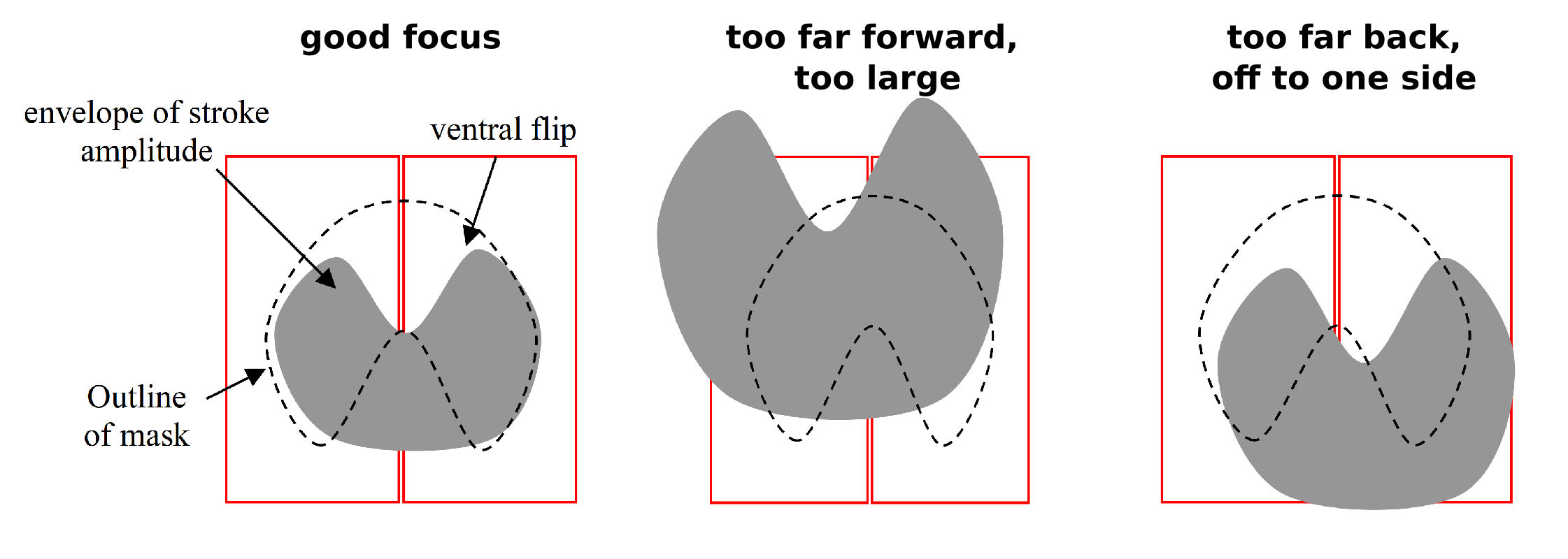
The IR wing sensor provides the analog signal to the wingbeat analyzer, which in turn detects the frequency and amplitude of the downstroke-upstroke reversal, also called the ventral flip. Proper fly alignment over the sensor is crucial – the wingbeat analyzer is a robust instrument and will report spurious values even if the input signal is messy.

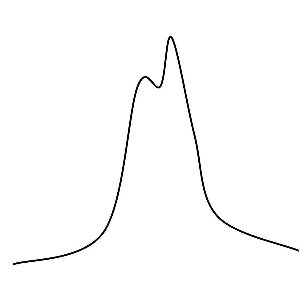
If the fly is properly focused over the sensor, then the resultant signal from both the left and right outputs of the wingbeat analyzer should look like this for each wing stroke:

Good hütchens

• Narrow waveform
• looks like a hat
• Looks like a little hat == hütchens
• quantal cycle-by-cycle amplitude pops
• Second peak larger than first

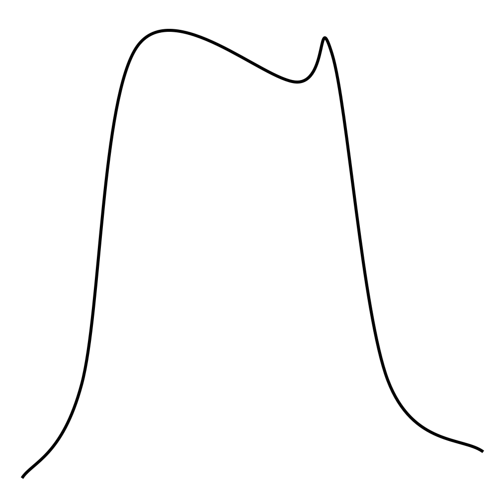
Bad Hütchens

• Broad waveform
• No cycle-by-cycle amplitude variation
• Saturated wing signal

It looks more like a lüdenhut (ask MD)

fly is likely too far forward over the mask

Bad Hütchens

• Narrow waveform
• Quantal cycle-by-cycle amplitude variation
• First and second peak equal height, or second is smaller

Fly is either too far away from the sensor surface, or too far from IR source, or both

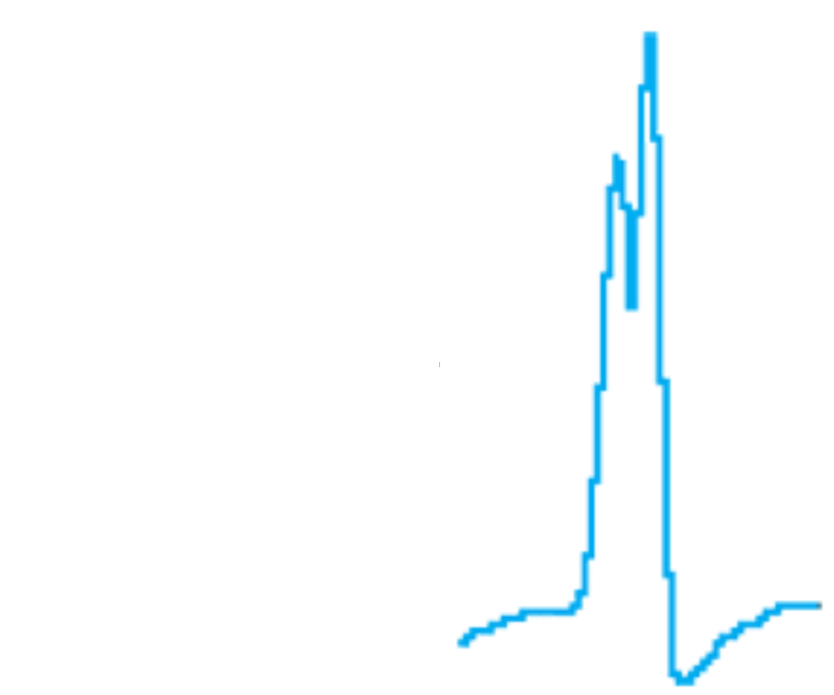
Good hütchens

Another example of good hütchens (screenshot from an oscilloscope)

Changes to the hütchens that come from moving the fly in the arena are best learned by experimentation. If possible, align the fly while presenting a closed loop stimulus (see below) such as a dark stripe for the fly to fixate on. Some general guidelines for aligning the fly are as follows:

• If there is no amplitude variation (the hütchens are not ‘bouncy’) the fly is likely too far forward. If the amplitude seems too small, increasing the gain, increasing the current from the IR LED, or moving the IR LED closer to the fly may help.
• If the left and right hütchens are not identical in shape, double check that the fly is glued symmetrically, is facing straight forward, and is centered under the LED and above the IR sensor. This can be difficult, but well worth the time spent, as it avoids later frustrations!
• If the wing hütchens disappear altogether or are saturating the wing beat analyzer, the fly is either too close to the IR LED and forward, or too far back and away from the IR LED, respectively.
• If fixing a stripe seems to be an issue for a (wild type) fly, adjusting left or right slowly and waiting for better fixation is probably necessary. By backing the fly up, lowering the gain, or reducing the current from the IR LED, you can also reduce the difficulty of fixating. To ensure proper alignment, these settings should not be different than those used in actual experiments.

The WBA tracks the analog wing sensor signal voltage, and measures a suite of parameters for each wing stroke (defined by the inflections in the hütchens occurring between the user-defined trigger and gate values):

Inputs

• Source: left or right wing to set Gate and Trigger
• Trigger: voltage threshold to detect peak of downstroke
• Gate: time frame to detect peak of downstroke
• Gain: amplification of hütchens – should read 2.5-3.5 Volts for standard DAQ
• Filter: low-pass filter analog sensor signals

Outputs

• Left: analog signal from IR wing sensor
• Right: analog signal from IR wing sensor
• Frequency: stroke frequency in cycles/sec
• L-R: left minus right amplitude - proportional to yaw torque
• L+R: left plus right amplitude - proportional to thrust
• Flip: a brief TTL pulse synchronized with the ventral flip
• Sync: a TTL pulse synchronized with each wing beat - used to trigger an oscilloscope sweep

Arena

LED flight arena: a modular array of 8x8 dot matrix LED panels. Each panel is independently addressable – i.e. can show a different visual pattern and can display 16 intensity levels (grayscale). In the typical 12 column circular configuration, each LED (pixel) subtends (no more than) ~3.5 degrees at the retina. The arena should be powered-up when the controller power switch is toggled (note that some odd behavior might occur depending on the order of powering equipment up).

Controller

The controller is the interface between the PC and the arena. The following notes document the newer, slimmer version (3.0) of the controller.

Signals available on the front panel of the arena controller v 3.0 with the newest controller code (v1.3):

• ADC0: analog input in mode 1 and 2 of channel x
  • This input should be in the form of L-R. That is, with a negative gain in modes 1 and 2, a negative signal will cause a decrease in channel frame and a positive signal will cause an increase in channel frame number.
• ADC1: analog input in mode 1 and 2 of channel y
  • This works in the same manner as ADC0
• ADC2: analog input in mode 3 of channel x
• ADC3: analog input in mode 3 of channel y
• DAC0: voltage proportional to current frame number (in the unit of volt) in mode 1, 2, 3, 4, and PC dumping mode of channel x, update analog output in mode 5 (debugging function generator) of channel x;
• DAC1: voltage proportional to current frame number (in the unit of volt) in mode 1,2,3, 4, and PC dumping mode of channel y , update analog output in mode 5 (debugging function generator) of channel y;
• DAC2: output from this channel is accessible from MATLAB, see the set_ao command
• DAC3: output from this channel is accessible from MATLAB, see the set_ao command
• Int0: unused;
• Int1: timing for fetching and displaying each frame when controller works in default mode and PC dumping mode. It is set to high before controller fetches a new frame data and reset to low when the controller finishes sending the data to the arena.
• Int2: laser trigger (see appendices for usage information)
• Int3: unused

The DAC0, and DAC1 voltages will be values between 0V…10V. The size of the voltage steps is set by the number of frames in X, Y for the current pattern (e.g. 96 frames in one channel would lead to voltage steps of 10/96V; frame index 48 would be roughly 5V). These outputs are consistent and can be used to recover the exact frame position for patterns of at least 500 frames (can only be done approximately for larger patterns). These instantaneous pattern positions are essential for off-line analysis of closed-loop behaviors, and are useful for validating open-loop experimental protocols.

Software Operation

Arena operation requires a MATLAB installation. The specific files necessary for interfacing with the controller can be downloaded from the Software Repository and added to the MATLAB path. This section contains an overview of the GUI components and functions, an introduction to software control of the arena, pattern building commands, pattern acceleration discussion, and SD flash programming instructions. Many of these concepts are rehashed in the example experiment section.

MATLAB GUI Control: PControl

Most of the arena functionality is accessible from the PControl GUI. It is a good place to start learning the system.

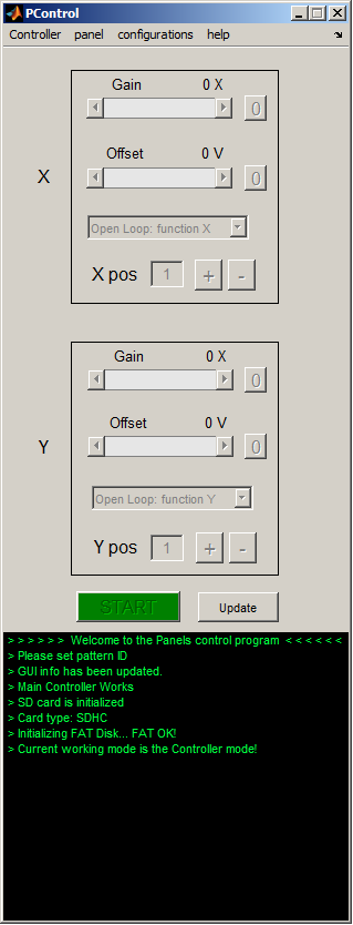
Quick Start

1. Switch on the arena. Panels will show addresses.
2. Insert pre-programmed SD flash card into the controller.
3. Switch on the controller. Verify that the left-hand green PWR LED is on steady. Arena will go dark.
4. Start MATLAB.
5. In the Command Window, type PControl.
6. Verify the serial connection between the PC and the controller, select: Controller → blink LED, verify the 2nd red LED for “Memory status” blinking on the controller.
7. Load a pattern in PControl with the menu Configurations → set pattern ID → Choose a Pattern from the dropdown menu.
8. First re-zero X and Y Gain and Offset. Set Gain to a non-zero value in the appropriate channel (X or Y), hit Start, and Stop.

Open-Loop operation

Once you have loaded a pattern to display in the arena, set the menu options in the X and Y front panel drop down menus to Open Loop: function X, and Open Loop: function Y (the default modes). Hit Start. Play with the Gain and Offset values at will. Can you figure out what X pos and Y pos do? Program a moving pattern by using the functions menu to load periodic waveforms. Now manipulate the Gain and Offset controls and hit Start.

Open Loop with an external waveform

From the patterns menu, load the checkerboard pattern (hopefully, it is Pattern Index 1). Connect the output of a function generator to ADC2. From the X drop down menu, select Position: ADC2 sets X ind. Set the X Gain and hit Start. Vary the controls on the function generator, and verify that the pattern moves in register with function generator output. Move the checkerboard pattern horizontally by loading an internal function in the Y-channel and selecting the drop-down menu Open Loop: function X.

Closed-loop operation

The closed-loop mode is similar to running the pattern in Open Loop with an external waveform. The only real difference is that the external function is a time-varying voltage proportional to the fly’s wing amplitude (i.e. steering torque). To give the fly control over the X pattern (e.g. load a single stripe pattern, which should occupy the X channel), plug the L-R Amplitude outputs from the Wingbeat Analyzer to ADC0. Set the X-channel drop-down menu to Closed Loop: ADC0 (L-R). Set the X Gain to a negative value, and hit Start. Use the X Offset to balance steering asymmetry. If you wish to run the Y pattern in closed-loop, connect L-R Amplitude to ADC1 and set the Y-channel drop-down menu to Closed Loop: ADC1 (L-R).

Introduction to software control from MATLAB

Events in PControl.m (controller GUI) are implemented as calls to Panel_com.m, a case structure of sub-functions used by the GUI. Anything the GUI can do may be executed on the command line (or in a script) with arguments to Panel_com(‘argument’, \[value\]). You can think of X and Y as axes of the memory buffer that stores the individual frames to display on the panels. For the arenas we constructed here, each frame of the display will be a 96×32 pixel bitmap (corresponding to the number of individual LED’s around the azimuth and zenith, resp. of the arena). X and Y correspond to the two dimensions of the array of frames, they do NOT necessarily correspond to the coordinates of the display with respect to the fly. Here’s an example: consider a vertical stripe rotating 360 degrees around the fly. This pattern requires 96 individual frames, one for each column of pixels such that if they are displayed sequentially, the pattern looks like a stripe rotating smoothly around the yaw axis. The 96 frames can be stored in X(1:96), Y(1). By contrast, consider a rotating striped drum with each black-white pair composed of 8 pixels. The pattern can be stored in only 8 frames, X(1:8), Y(1), and simply iterated to evoke the perception of a pattern moving smoothly around the yaw axis.

In general, you use PControl and associated functions to design, build, and test the patterns for experiments. Then, you execute individual functions in scripts to conduct a controlled, repeatable experiment. For example, Panel_com is a function with a series of different arguments – anything you do with PControl (and some things you cannot) may be programmed by Panel_com on the command line. Here are some examples:

Panel_com('set_pattern_id',4); % load pattern number 4 from SD
Panel_com('set_mode',\[1,0\]); % closed-loop mode "Closed Loop: ADC0 (L-R)"
Panel_com('set_position'\[49, 1\]); % set the position to X=49,Y=1
Panel_com('send_gain_bias'\[12,0,0,0\]); % send Gain and Bias values
Panel_com('start'); % begin pattern motion
pause(20); % let the pattern run for 20 seconds
Panel_com('stop'); % stop pattern motion

Panel_com commands are detailed in Technical Appendix 1.

Example Experiments

Building a pattern file

The display of visual patterns requires three separate steps: First, patterns must be created in numeric form most typically using a convenient program such as MATLAB, and saved in a suitable format. Second, this file, containing the display information, is burned onto an SD (flash memory) card from a computer. Third, the SD card is inserted into the Arena Controller, and the contents are sent to the panels using the Controller’s software (using low-level, C code, featuring deterministic timing).

Although involving many steps, this process is straightforward, especially if using our provided MATLAB functions that make this first step easier. The most complicated part for the user is constructing the arrays that contain the display information for the panels in the arena. In doing so, it is important to keep several concepts in mind. The number of unique panels required for a display may vary. Each 8x8 pixel panel is given an identity, which is set using the procedure described below. When you power up the arena, these IDs are displayed on each panel. The identities may or may not be unique. The most flexible experimental setup will require unique panel IDs. It is important to recognize that the way you create a pattern will depend upon the number of unique panels in your arena and their spatial distribution.

The critical step in creating a pattern file in MATLAB is using the make_pattern_vector command, which operates on a pattern structure. The pattern structure has the following critical fields that are required before the structure may be saved in an *.mat file and loaded on the flash card:

• pattern.x_num: the number of frames in the x channel
• pattern.y_num: the number of frames in the y channel
• pattern.num_panels: number of unique panel IDs required
• pattern.gs_val: grey scale value; must be either 1, 2, 3, or 4.
  • 1 indicates all pixel values in pattern.Pats are binary (0 or 1)
  • 2 indicates all pixel values in pattern.Pats are either 0, 1, 2, or 3.
  • 3 indicates all pixel values in pattern.Pats fall in the range of 0…7.
  • 4 indicates all pixel values in pattern.Pats fall in the range of 0…15.
• pattern.row_compression: 0 or 1. This sets the simplest available compression mode. When set to 0, you produce a pattern as normal, with 8×8 pixels per panel. With row compression enabled (=1), the patterns are 1/8 the size, and are designed as 1×8 pixels per panel. These patterns are at least 5× faster.
• pattern.Pats: This field contains the basic data for the displayed images.
  pattern.Pats is a matrix of size (L,M,N,O), where:
  L is the total number of pixel rows
  M is the number of pixel columns
  N is the number of frames in the x direction, same as pattern.x_num
O is the number of frames in the y direction, same as pattern.y_num
  Thus, each entry in this L×M×N×O matrix is either one bit (for pattern.gs_val=1), 2 bits (for pattern.gs_val=2), 3 bits (for pattern.gs_val=3), or 4 bits (for pattern.gs_val=4). For example, for pattern.gs_val=3, each pixel value can be set as 0…7, where 0 is OFF, 7 is maximal ON, and the intermediate values linearly scale this intensity. Most of the work in generating a display pattern is in creating the pattern.Pats matrix. However, if a simple azimuthal shift is required (as in a yaw control experiment), the function ShiftMatrix.m can be used to create shifted maps required to depict the moving image.
• Pattern.Panel_map: this is a vector or matrix that encodes the orientation of the panel IDs.
  See notes above for why this is important. A simple example might be:
  Pattern.Panel_map = \[1 2 3 4 5 6 7 8 9 10 11 12\];
  For a case where columns of panels display the same information. The standard Panel_map for a 48 panel, 12 column arena is:
  

  pattern.Panel_map = \[ 12 8 4 11 7 3 10 6 2 9 5 1 ; ...
  24 20 16 23 19 15 22 18 14 21 17 13; ...
  36 32 28 35 31 27 34 30 26 33 29 25; ...
  48 44 40 47 43 39 46 42 38 45 41 37 \];
  

  Here every panel in a 12x4 panel arena has a unique address. The Panels should be addressed starting from 1, and going up to pattern.num_panels. The reason for this peculiar sequence of panels is that in the v3.0 panel hardware, we use 4 I2C buses, and we want consecutive panel ID’s to be placed on each of the 4 busses (find the 1, 2, 3, 4, etc. and notice that these are shifted by 3 columns).

• pattern.BitMapIndex: a structure that encodes the spatial panel IDs.
  This field can be generated using the function, process_panel_map.m, which operates on pattern.Panel_map, e.g. pattern.BitMapIndex = process_panel_map(pattern);
• pattern.data: vector format of the data.
  The final vector form of the data that is ready for output can be created using pattern.data = make_pattern_vector(pattern); . The resulting structure is then saved as a *.mat file.

Here is an example MATLAB script that uses these functions to create a simple panel file for a stripe fixation experiment:

clear all;
pattern.x_num = 96; % 96 frames in X, one per pixel along arena circumference
pattern.y_num = 1; % pattern does not use Y channel
pattern.num_panels = 48; % designed for complete 48 panel arena
pattern.gs_val = 1; % pattern uses 2 intensity levels
pattern.row_compression = 1; % use row compression

% Initial pattern is just one stripe of 8 off pixels
% because we are using row compression the pattern size if just 4 pixels ×
% 96 pixels. We only need to specify one row of pixels per panel
InitPat = ShiftMatrix(\[ones(4,88) zeros(4,8)\], 1, 'r', 'y');

% create Pats as an array sized to hold complete pattern
Pats = zeros(4, 96, pattern.x_num, pattern.y_num);

% frame 1,1 of the Pattern is the Initial Pattern
Pats(:,:,1,1) = InitPat;

% fill in the remaining X positions by shifting each subsequent frame to
% the right by 1 pixel.
for j = 2:96
    Pats(:,:,j,1) = ShiftMatrix(Pats(:,:,j-1,1), 1, 'r', 'y');
end

% map this pattern onto the 48 panel standard arena
pattern.Pats = Pats;
pattern.Panel_map =  [  12  8   4   11  7   3   10  6   2   9   5   1 ; ...
                        24  20  16  23  19  15  22  18  14  21  17  13; ...
                        36  32  28  35  31  27  34  30  26  33  29  25; ...
                        48  44  40  47  43  39  46  42  38  45  41  37];

pattern.BitMapIndex = process_panel_map(pattern);
pattern.data = Make_pattern_vector(pattern);

% store the pattern
directory_name = 'C:\matlabroot\Patterns';
str = [directory_name 'Pattern_2_stripe_48P_RC']
save(str, 'pattern');

Accelerating your patterns

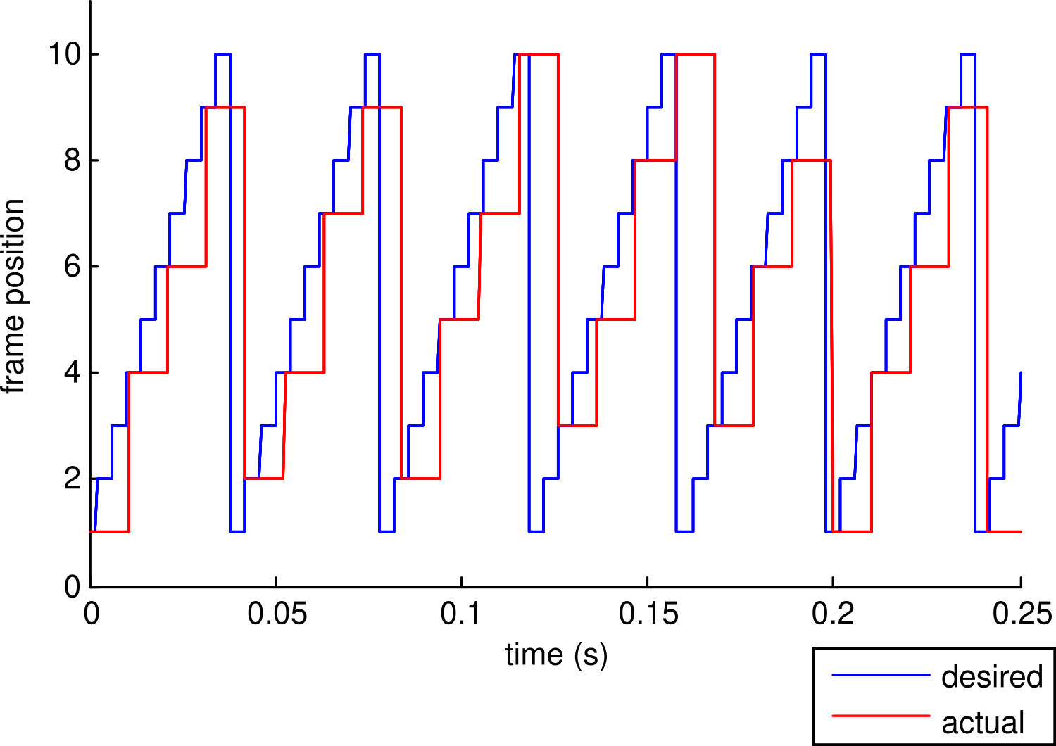
Let’s face it, we all like speed. All the fancy things that one can do with the controller will usually incur a cost—the patterns will probably display slower. By slower, we mean that the controller will spend more time refreshing an individual frame, and thus to keep up with the expected display rate (either set in open-loop by the function generator, or in closed-loop by the fly), the controller will drop frames. Suppose that we want the controller to display a 10 frame pattern at 250Hz, but the maximum achievable frame rate is 95Hz. The figure on the right should give a rough idea of the actual sequence of displayed frames as compared to the desired sequence.

How do you know your maximum achievable rate? Benchmark your pattern. This can be done automatically using the controller and the results are visible in PControl. A quick and rough benchmark can be performed by manually increasing the display rate and observing when the skip-indicating LED (green one, next to the power on LED in the middle of the controller box) starts to blink.

How does one get more speed?

1. Simplify the pattern. Either don’t use grayscale, reduce the number of panels used, or update the arena configuration to disable a subset of the panels in your arena (e.g. you can mask out the top and bottom row and just drive your pattern in the central 2 rows along the equator of the flies’ eye).
2. Use row compression. A large number of patterns we might care to try consist of identical pattern data for all rows of the pattern. When this is the case, a row-compressed pattern will just consist of one row instead of 8. This results in a speedup factor of at least 5. To enable row compression, simply make a pattern with only one row per panel, and include the setting (pattern.row_compression = 1;) in the pattern making script. See example above.
3. Use ‘identity’ compression. The general method outlined for making and sending patterns is simple (elegant, perhaps) but should strike no one as optimal. Many patterns contain large swaths of pixels that are simply on or off. One simple shortcut that has been implemented is to simply send the row-compressed version of the panel data for a panel that corresponds to a pattern piece that is all one value (works for grayscale too!). This feature is not used at pattern making time, but rather while the pattern is running. Identity compression can be enabled by invoking: Panel_com('ident_compress_on') from MATLAB. Seems like a brilliant idea, why isn’t it just always on? This brings up an important lesson in compression—there are no one-size-fits-all solutions. Sure this methods speeds up the pattern containing a single stripe, but consider a striped drum pattern—all of the extra comparisons needed to determine if a particular panel’s piece of the pattern can be sent as a single row, will slow things down considerably and never find a compressible pattern patch.
4. Use super-speed mode where for small patterns with few frames, the data can be stored locally on the panels.
5. Think outside the box… Each pattern can probably be optimized in its own way.

Programming the SD Flash Card

The SD card is where you store patterns and functions for running the arena. These are programmed onto the SD card using PControl and then moved to the Controller.

1. Once you have a collection of patterns that you wish to display in the arena, put them all into C:\matlabroot\patterns\. You may in fact put them any place you wish, but this is the default directory.
2. Plug a SD Flash card into a port, using a USB card reader. Verify that it appears as a drive letter (usually E).
3. In MATLAB, run PControl, and select configurations → load pattern to SD.
4. In the Pattern Selection window, press Add Folder, navigate and select the folder storing your pattern files. You may also individually add the patterns, if this becomes time consuming to achieve the correct order of patterns, consider naming each pattern as Pattern_##_id where ## is the number you wish the pattern to be and id is an identifying name. This will ensure the patterns in the folder selected are added in the correct order
5. Hit OK.
6. In the Pattern Selection Tool window, verify the patterns you want to store.
7. Press Make Image, then Burn. If you are prompted for the drive letter at any time, type it into the prompt and press OK.
8. DO NOT take out the SD card until you see a message confirming that the SD card writing is finished.
9. Plug the SD card into the arena controller. You may need to turn the controller off and on for it to recognize the card correctly.
10. To test the pattern, open up PControl and select configurations → set pattern ID → your pattern (from the dropdown menu). Now you can use the PControl GUI to run your pattern by selecting values and pressing the start button.

To be able to automatically access the patterns on an SD card from the PControl GUI, you must be using the SD on the same machine on which it was programmed. If you need to load patterns from an SD card programmed onto another machine (or if you see that patterns and/or functions copied onto the card behave strangely, you should synchronize the SD information from the card to your PC by clicking on the controller → sync SD info menu items in the PControl GUI.

Loading Functions to SD card

The process for storing functions onto the SD card is similar, except you use configurations → load functions to SD. It is best to program all patterns and functions you will need for your experiments onto the SD card and then move it over to the controller.

Loading Arena Configurations to SD card

The process for storing arena configurations onto the SD card is similar, except you use configurations → load config to SD. This document currently does not explain arena configurations, but these are a critical aspect of running the v3.0 arena. For these exercises, use the default configurations provided for you.

Original file

This user guide is an online version of the original flight simulator user guide (available for download in the original file format).

---

Table of contents

• Technical Appendix